13.1 One-Sample: Hypothesis Testing on the Mean

We will consider testing:

$$H_0: \mu = \mu_0$$ $$H_1: \mu \not= \mu_0$$

Let $x_1,x_2,\ldots,x_n$ be a random sample for a normal distribution with unknown mean $\mu$ and unknown variance $\sigma^2$.

If the null hypothesis $H_0: \mu=\mu_0$ is true, the random variable

$$T=\dfrac{\bar{x}-\mu_0}{\hat{s}/\sqrt{n}}$$

has a $t$ distribution $n-1$ degrees of freedom.

13.1.1 Example

A company wants to improve sales. Previous sales data indicate that the mean sale was 220 euros per transaction. After training the sales force, recent sales data were taken from a sample of 9 salesmen. The company needs to know if the training had worked.

Solution

• Data

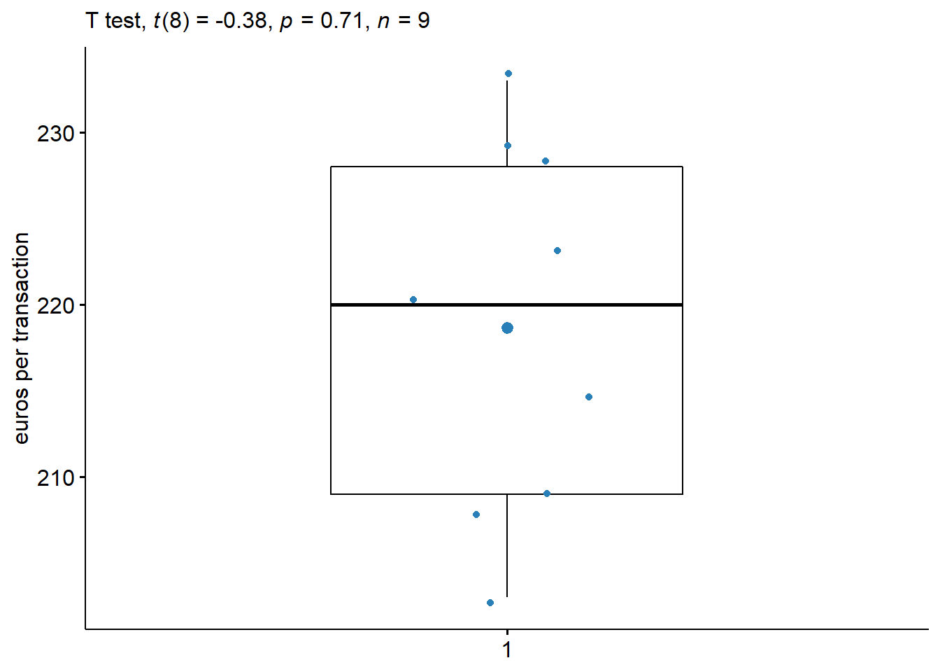
$$x= \{ 203, 229, 215, 220, 223, 233, 208, 228, 209 \}$$

$$n=9; \,\,\,\, \bar{x}=218.67 ; \,\,\,\, s = 10.52.$$

• Hypothesis

$$H_0: \mu = 220$$ $$H_1: \mu \neq 220$$

• Test statistic

$$T=\dfrac{\bar{x}-\mu}{S/\sqrt{n}} = \dfrac{218.67-220}{10.52/\sqrt{9}}= -0.38$$

• Decision

• Critical Value

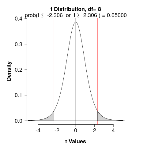
We would reject $H_0$ if $T$ were less than $t_\alpha$ or greater than $t_\alpha$ (determined used a $t$-table)

$$\alpha = 0.05; \,\, df = 8$$

The test statistic $T= \pm 0.38$ is not less than $t_\alpha= - 2.31$ nor greater than $t_\alpha= \pm 2.31$. Then, we fail to reject the null hypothesis. That is, the test statistic does not fall in the critical region.

• p-value

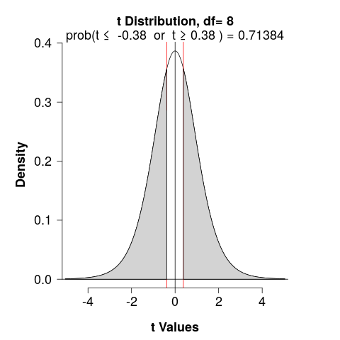
We would determine the area under a $t_{df}$ curve, to the right of $T$ and to the left of $-T$

$$T = \pm 0.38; \,\, df = 8$$

The $p$-value of the test is 0.71, which is greater than the significance level $\alpha = 0.05$. Then, we fail to reject the null hypothesis. The conclusion is the same regardless of the approach use.

• Interpretation

There is insufficient evidence, at the $\alpha= 0.05$ level, to conclude that the mean sale is not different from 220 euros (per transaction).

• Reporting

A one-sample t-test was computed to determine whether the mean sales was different to the population normal mean sales (220).

Your turn

• The company thinks that there is a difference (that the mean sales increased after the training). Test this hypothesis.