16.10 Quadratic Models
In a single linear regression we can include the squared term of the independent variable, that is \(x^2\). In that case, the model is call second-order model. The quadratic term \(x^2\) enable us to hypothesize curvature in the plot of response model relating \(y\) to \(x\).
A quadratic (second-order) model in a single quantitative independent variable is
\[ y_i = \beta_0 + \beta_1 x_i + \beta_2 x_i^2 +\epsilon_i\]
where
- \(\beta_0\) is the (\(y\)-)intercept of the curve.
- \(\beta_1\) is a shift parameter.
- \(\beta_2\) is the rate of curvature.
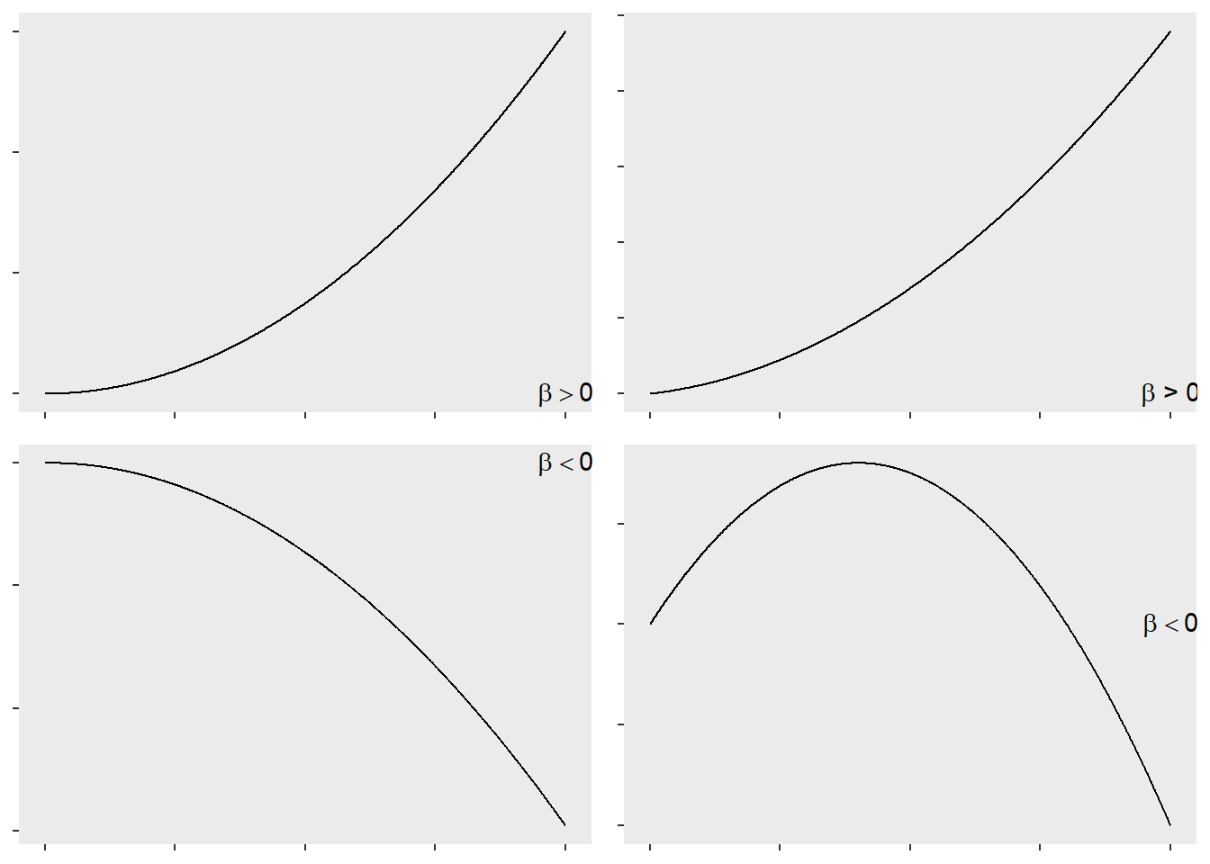
When \(\beta_2\) is positive, the curve opens upward. When \(\beta_2\) is negative, the curve opens downward.
16.10.1 Example
The data shows the number of weeks employed and the number of errors made per day for a sample of assembly line workers. Find a 2nd order model, conduct the global F–test, and test if \(\beta_2 \neq 0\). Use \(\alpha = 0.05\) for all tests
| errors | 20 | 18 | 16 | 10 | 8 | 4 | 3 | 1 | 2 | 1 | 0 | 1 |
| weeks | 1 | 1 | 2 | 4 | 4 | 5 | 6 | 8 | 10 | 11 | 12 | 12 |
| Source: cStatistics for Business and Economics, Global Edition. Chapter 12 |
The model to be fitted is \(\text{Errors}_i= \beta_0 +\beta_1\text{Weeks}_i + \beta_2 \text{Weeks}_i^2 + \epsilon_i\)
| Observations | 12 |
| Dependent variable | errors |
| Type | OLS linear regression |
| F(2,9) | 174.062 |
| R² | 0.975 |
| Adj. R² | 0.969 |
| Est. | 2.5% | 97.5% | t val. | p | |
|---|---|---|---|---|---|
| (Intercept) | 23.728 | 21.205 | 26.252 | 21.269 | 0.000 |
| weeks | -4.784 | -5.747 | -3.821 | -11.237 | 0.000 |
| weeks2 | 0.242 | 0.171 | 0.313 | 7.715 | 0.000 |
| Standard errors: OLS |
The fitted model is
\(\widehat{\text{Errors}}_i= 23.728 - 4.784\text{Weeks}_i + 0.242 \text{Weeks}_i^2\)
- Considering \(F(2,9) = 174.062\) with $ p-value = 0.000$, \(F\)-test indicates at least one parameter is different from zero.
- Considering \(t(\beta_2) = 7.715\) with $ p-value = 0.000$, \(t\)-test for \(\beta_2\) indicates indicates curvilinear relationship exists.